Introduction
If you are/were interested in Hearthstone, its metagame and its “data” you probable know about vicioussyndicate (vS)
Among the data they provide probably one of the most interesting is the “Meta Score”
From their F.A.Q.
Q: What is the meaning of the Meta Score and how do you compute it?
The Meta Score is a supplementary metric that measures each archetype’s relative standing in the meta, based on both win rate and prevalence, and in comparison to the theoretical “best deck”.
How is it computed?
…
We take the highest win rate recorded by a current archetype in a specific rank group, and set it to a fixed value of 100. We then determine the fixed value of 0 by deducting the highest win rate from 100%. For example, if the highest win rate recorded is 53%, a win rate of 47% will be set as the fixed value of 0. This is a deck’s Power Score. The range of 47% – 53%, whose power score ranges from 0 to 100, will contain “viable” decks. The length of this range will vary depending on the current state of the meta. Needless to say, it is possible for a deck to have a negative power score, but it can never have a power score that exceeds 100.
We take the highest frequency recorded by a current archetype in a specific rank group, and set it to a fixed value of 100. The fixed value of 0 will then always be 0% popularity. This is a deck’s Frequency Score. A deck’s frequency score cannot be a negative number.
We calculate the simple average of a deck’s Power Score and Frequency Score to find its vS Meta Score. The vS Meta Score is a deck’s relative distance to the hypothetical strongest deck in the game. Think of Power Score and Frequency Score as the coordinates (x, y) of a deck within a Scatter Plot. The Meta Score represents its relative placement in the plane between the fixed values of (0, 0) and (100,100).
If a deck records both the highest popularity and the highest win rate, its Meta Score will be 100. It will be, undoubtedly, the best deck in the game.
The final result usually looks like this
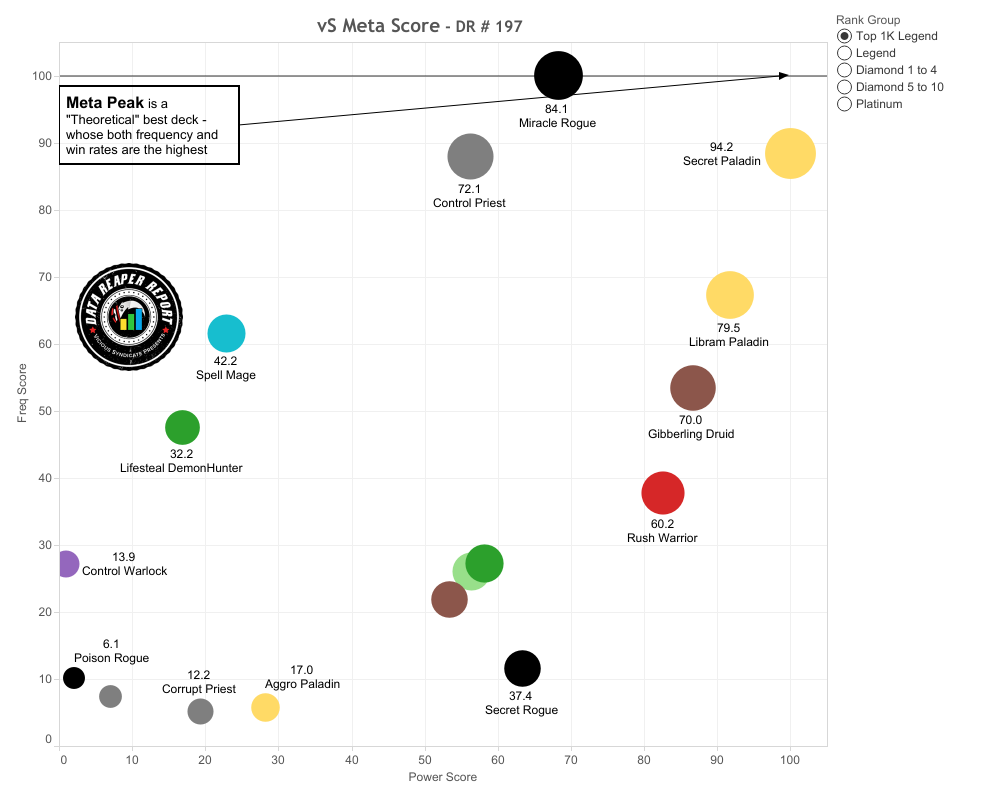
The size of the circles represent the meta score, the bigger it is the bigger the value.
Now, before asking ourselves to translate this methodology in LoR, what’s the theory behind the Meta Score?
The Meta Score, in this case a LoR-Meta Index (LMI) is an extremely simple example of a Composite Indicator (CI).
A composite indicator is the result of combining multiple variables usually into a single value. If you ever heard of a ranking among cities / companies / universities, and so on, chances are that it’s done with a Composite Indicator.
In my opinion, even among other statistic’s fields, creating a CI is more like an art. There is no perfect indicator (as there’s no perfect model ) at most there good and bad indicators. Even if their creation can be entirely data driven, most of the works stem from a theoretical framework that it’s very subjective. There are 10 main steps and each one of them can highly change the overall result. This doesn’t mean that one can’t trust a CI, there are ways of checking the quality of a CI but that’s almost an entirely problem I won’t tackle for this case-study.
While building a CI can be quite the challenge, creating a LMI is not as hard as some of the required steps are (in this case) not necessary or quite simplified.
Defining our parameter of interest (Framework)
The objective of the CI is to measure the “strength” of the current meta decks. Usually the context and more details are added but overall that stength is a combination of “win rates”, “play rates”, “consistency” and probably other variables I don’t remember here, in the context of LoR I would probably add something like maybe “the ability to interact with the opponent”.
The definition I’ll use is the following
The performance of a deck is defined by its own strength and popularity inside the metagame.
Data selection
Sadly, for now, this step it’s way simplified: to measure the strength I’m going to use the win rate and to measure the popularity I’ll use the play rate. 12
The variables have been selected, but what about their values? Do we keep everything or filter them? To check this point let’s try to simply compute the LMI and take the 10 highest values without filters. (Fig. 1)
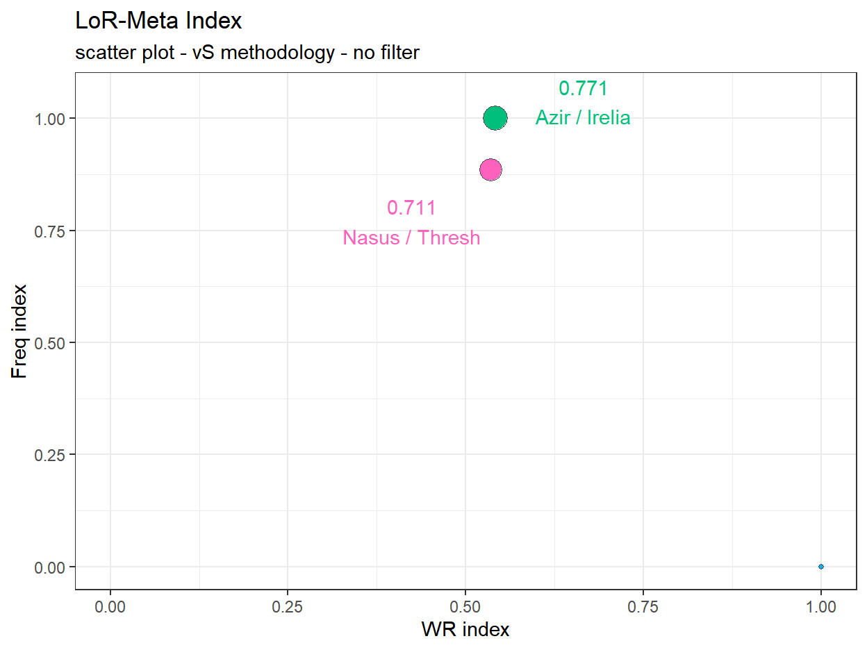
Figure 1: LMI no filter
While it may seems like there’s an error, sadly the graph is not wrong. If we keep all data (Appendix 1 ) , aside for the first 2 values of the LMI (corresponding to Nasus/Thresh and Azir/Irelia) the remaining 8 points are all at the coordinate (0,1) with Meta Score of 0.5.
Without filtering we left the outlier cases of 100% WR decks that also have a very small playrate. With this the “WR index” correspond the raw WR3 and just the frequencies are modified.
In order to find just the third point that’s not an outlier, we have to reach the 72° deck (Draven/Ez with a meta score of 0.45). While some choices about how to measure the index could deal with these extreme cases it’s not a good choice, it’s best to remove them from the start. Let’s try to remove the cases with less than 100/200/300 games.
A quick look at the summary (below) of WR suggest that 200/300 gives similar results. Looking at PlayRate doesn’t really makes sense as the value is directly tied to the number of games played.
Summary with Filter at 100:
   Min. 1st Qu.  Median    Mean 3rd Qu.    Max.
 0.2077  0.4182  0.4580  0.4512  0.4932  0.6229
Summary with Filter at 200:
   Min. 1st Qu.  Median    Mean 3rd Qu.    Max.
 0.2995  0.4356  0.4695  0.4614  0.4965  0.5827
Summary with Filter at 300:
   Min. 1st Qu.  Median    Mean 3rd Qu.    Max.
 0.2995  0.4358  0.4688  0.4603  0.4956  0.5827
To help me deciding I also created the Meta-score plots with the vS methodoly at the 3 benchmark for the filter.
Note: the following plots only needs to give an idea about the distribution of the decks on WR and Play Rate. The specific values for each deck are not of interest here.
Testing Filters
Filter at 100
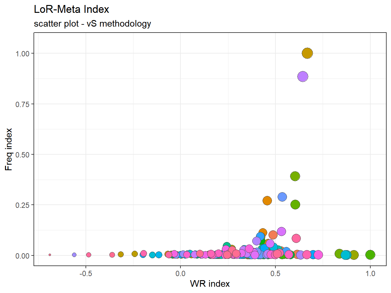
Figure 2: LMI filter at 100 (vS)
Filter at 200
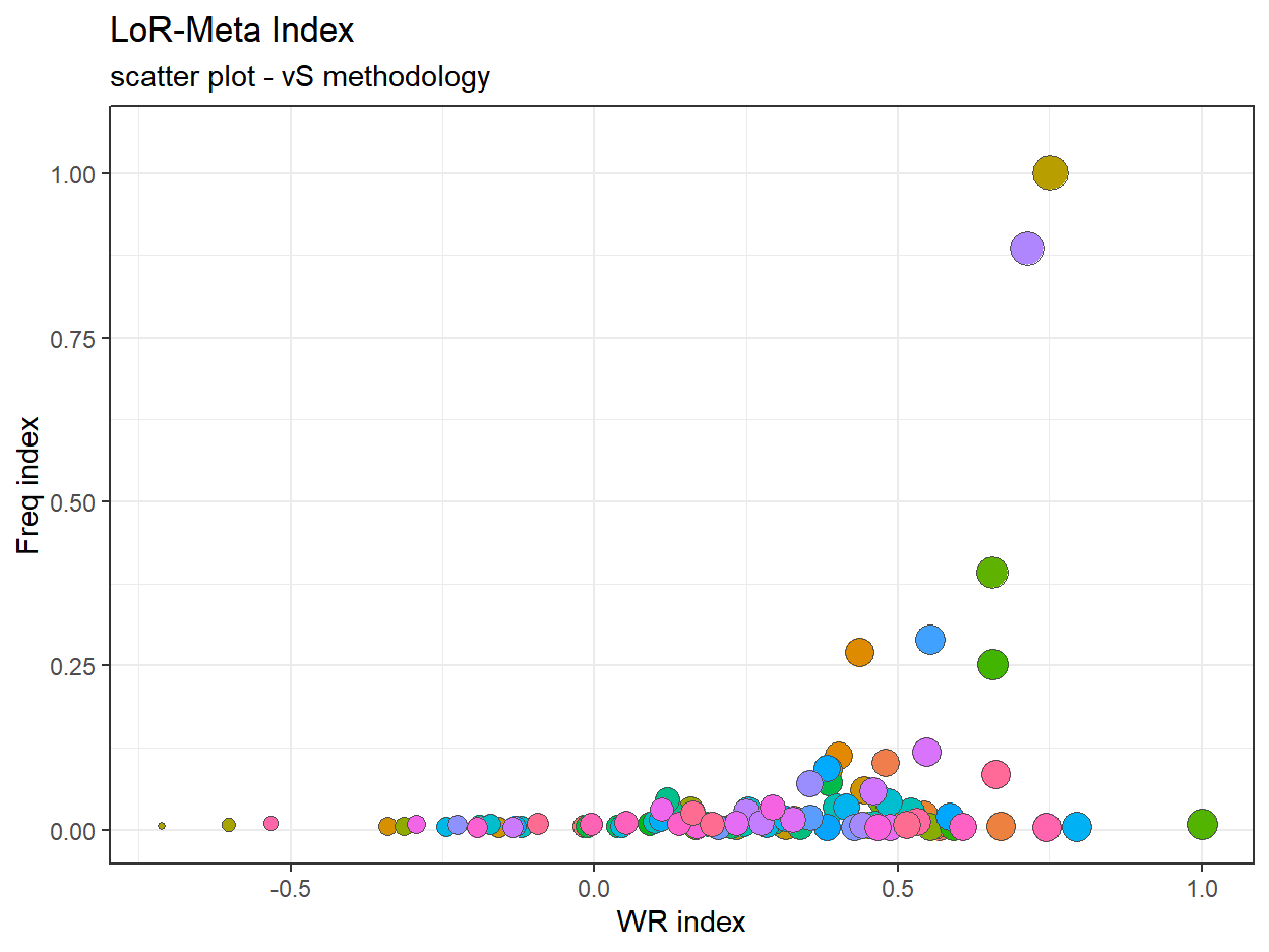
Figure 3: LMI filter at 200 (vS)
Filter at 300
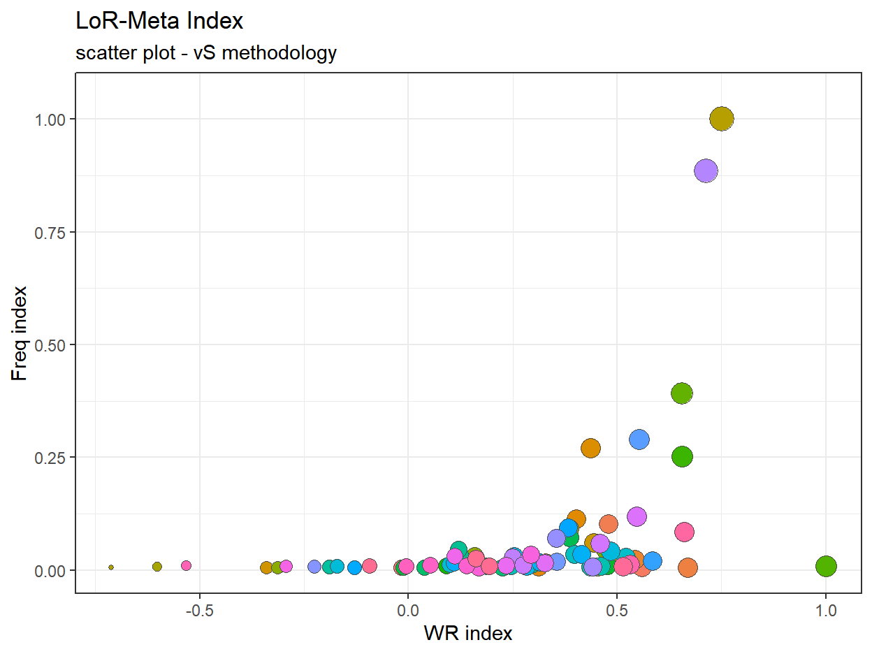
Figure 4: LMI filter at 300 (vS)
The first thing that comes to notice is that no matter what there are probably too many values near 0 of the Freq Index. This will be important in the next steps.
Overall, there are some minor changes jumping from 100 to 200 games min and a bit less from 200 to 300.
Filtering at 100 games may be too low as benchmark as the values are still too sensible to the sample size.
300 games seems ok but may be too harsh at removing “sleeper decks”, one need to consider that the sample sizes of LoR - Master rank data are not that high, so now it the filter may be too harsh, for now.
Also, worth noticing, the point’s radius doesn’t seems to change much for the plotted points and the radius here is proportional the LMI suggesting that the range of the index (for positive values) is a bit limited and it is confirmed when looking at the tabular data. (Appendix 2 )
So are we done? No, we haven’t even started. Let’s explain the following point to consider when creating a CI.
Normalization
Normalization usually refer to the process of rescaling a variable so that its domain is [0,1]
To compute the vS Meta score we don’t use the raw values of WR and playrate but the rescaled ones obtained following the rules described at the start. Usually this is done in order to bring the different variables to a more common scale, and, from a certain point of view the raw data are already like that, or at least they have theoretically the same range, but, their effect range is quite different and so is their variability.
In order to understand the value (and necessity of this process) it’s better to also show what would have been the results without such process.
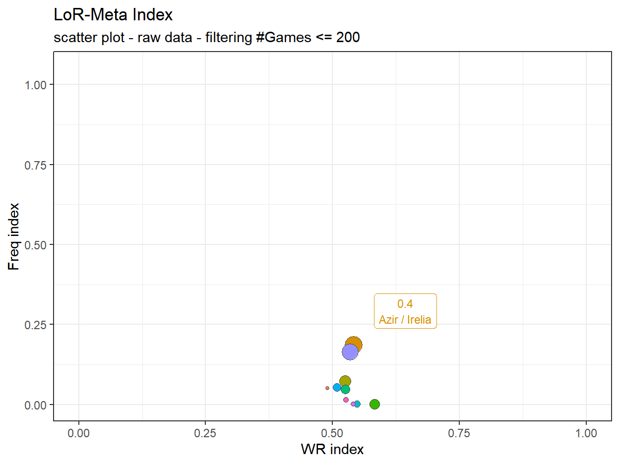
Figure 5: LMI with no Normalization
From 5 it’s possible to see how, without normalization, we are completely at the mercy of the raw data and their “limitations”.
For WR we have the problem that the values are limited to a small interval.
For Play rate not only it’s limited to a small interval but the data are quite skewed too with an heavy right tail and everything else concentrated around of the 0.005. This is most likely a sistematic problem in the data compared to HS, at least looking at vS. In their latest meta report (#197) even the smallest (reported) archetype have a decent 2.62% play rate. Sure there are many more decks that have a lower playrate but still the distribution looks less skewed without a huge discrepancy from the top.
The variables’ limitation is reflected of course in the LMI. See Fig. 6 to compare the LMI distribution with and without normalization and Table ?? to consult the data without normalization.
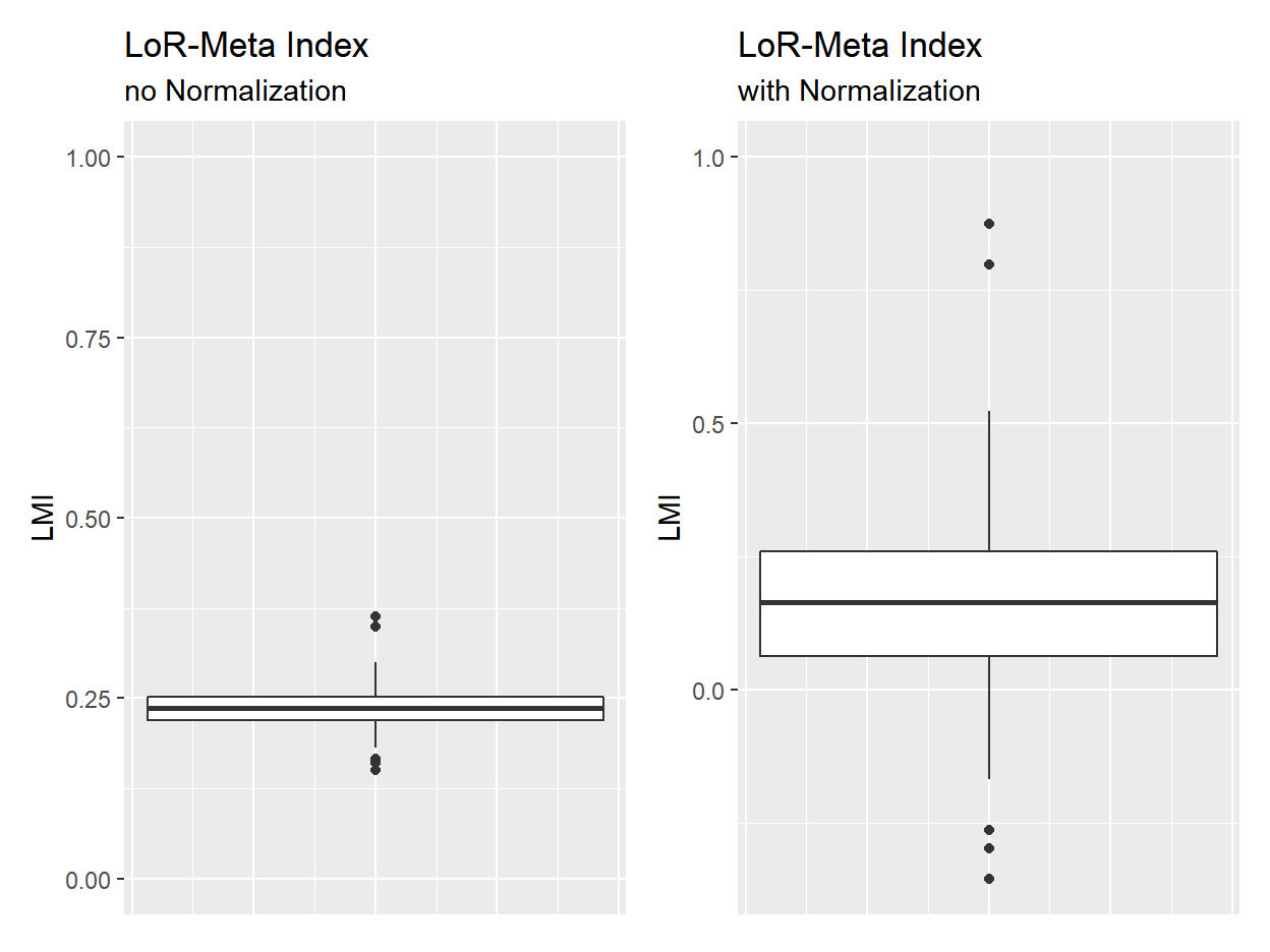
Figure 6: Comparing LMI distribution with and without normalizazion (vS methodology)
It can be seen the normalization here allows for a wider range of values being able to discern better the differences between each deck. As written at the start, it’s not that without normalization the index is not working as intended, that the index is wrong, but it’s not doing a good job, it’s a bad index. So, now that the role of normalization is clearer, how is it done? The choice is actually tied with the following step but here are the most common methods:
- Min-max: \(I_i= \frac{x_i - max(x)}{max(x) - min(x)}\) the min and max value are 0 and 1, everything else is scaled between them
- Standardization \(I_i = \frac{x_i - \mu_x}{\sigma_x}\) centered around the mean and with standard deviation equal to 1
- Distance to a reference \(I_i = \frac{x_i}{x_c}\) each value is the ratio against a reference value
- Rank \(I_i = rank(x_i)\) self-explanatory
- Quantile empircal distribution \(I_i = \frac{rank(x_i)}{N+1}\)
and so many more.
The normalization used for the vS-Meta score are modified example of of the min-max normalization. For the “Freq Score” there’s almost no difference from minmax as long as there’s a value with playrate almost equal to 0. For the “Power Score” (WR Index) the “min” and 1-max(WR) instead of the min(WR) in the data. I think the reason for using such method for the Power Score, is as follows: while by itself the distribution of WR is overall quite good. it wouldn’t be surprising if top decks had a win rate too much similar so limiting the effect of the power-score.
MinMax Normalization
The resulting values of the Freq Index are the ones I’m more interested too see how how they are affected by the normalization.
In addition to testing the rescaling to the raw values I’ll also test with the log-transformation and root-squared-transformation (sqrt) of playrate in order to deal with the high unbalance of its values. I’m aware that both transformations are not scale-invariant and for some people it may give too much value to deck with a small playrate.
Yet, not being stuck with scale-invariant processes is really limiting and I think this is a point worth considering in the context of Legends of Runeterra (and MtG most likely). In LoR decks are created around champions and regions, so the possible combinations are quite a lot and many of these can be good without being “meme decks”. This is the sistematic problem mentioned before this section and it means that the game is bound to be filled of decks with small playrates deck and only a selected few with a very high value resulting in a distribution that’s very right tailed.
I’ll start by showing the different distribution on Freq Index (Fig. 7) and then showing the resulting LMI (Fig. 8)
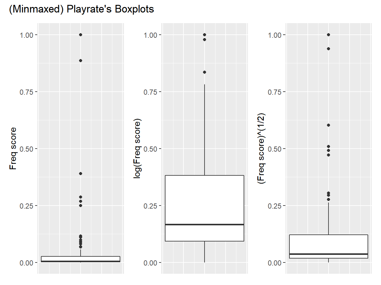
Figure 7: Boxplot of Freq Index when applying minmax normalization to: raw values / log-transformation / sqrt
The log-transformation seems to reduce well the skewness, the question is if it reduce it too much and the sqrt is more appropriate for this case study. I computed LMI for each case (Appendix 3) and looked at the LMI distribution (Fig. 8)
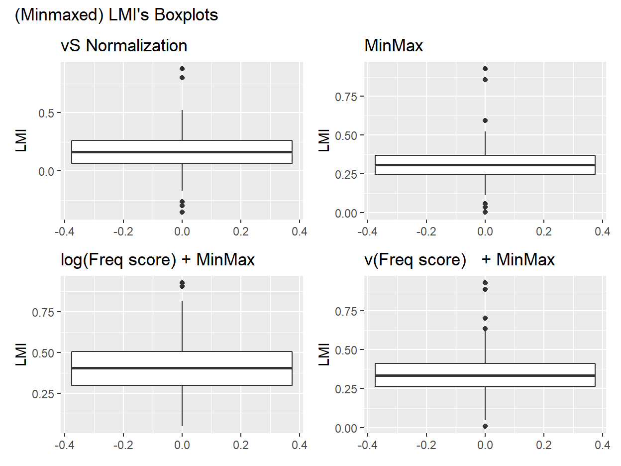
Figure 8: Boxplot of LMI when applying: vS / minmax / log trasnformation + minmax / sqrt + minmax
Compared to the vS-methodology, just using the minmax normalization gives the most similar results. When using the log or sqrt transformation of playrate all the values of LMI are bigger, which is as expected as we don’t penalize as much small playrates. Again, There is no correct answer, it depends on what’s the objective of the index. For example if we wanted to limit the results to just the top n highest decks, not adding a transformation may actually be more interesting as we would see bigger differences. Since I want to convey all the values then reducing the skewness may be more appropriate and would opt for the log-transformation.
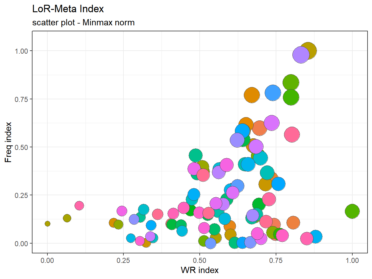
Figure 9: LMI / filter at 200 / log-tranformation of playrate / Minmax normalization
In the scatter plot it seems that the main “aestetic” difference is that the points are more aggregated to the right side of the chart because of all the high values of WR index. It’s not like this is wrong and it’s sort of obvious that the highest values of LMI correspond at high values of WR. Compared to the vS-methology it’s also possible to notice an higher variance of LMI among the top values. This approach seems to work “better” overall.
Quantile normalization
Note: instead of the proper formula, I’ll use \(I_i = \frac{rank(x_i)}{N}\). The reason being so that the highest value is always 1.
When using the quantile normalization, boxplots and other summaries of the transformed distributions are useless since such normalization will result into a uniform distribution. (Fig. 13 )
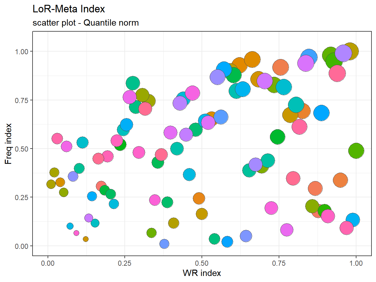
Figure 10: LMI / filter at 200 / Quantile normalization
I actually like this result compared to the minmax one. While the obvious critique is that decks like Azir/Irelia and Nasus/Thresh are not “a class of their own” like the raw data suggest (high WR but also extremely high playrate) this methodology not only cover well the spectrum of values for LMI but also for WR and Freq. Since it can further be improved I’ll continue now with the next steps using the Quantile normalization.
Another type of normalization is working with ranks. But since that directly translate in the following steps I’ll cover it later.
Aggregation (and weighting)
This step comprehend two equally important procedures: Decide how the importance/relevance of each variable when computing the index and how to aggregate those values.
Regarding the weighting we can’t really do that much. Either we opt for the same weight (0.50/0.50) without changing anything from the current metholody or the opt for any other justified convex combination.
Since in my opinion the Win rate is more important than play rate to measure the strength of a deck I’ll try assigning the (0.75,0.25) and (\(\frac{2}{3}\),\(\frac{1}{3}\)) more as a test. If people are interested in this topic I may try to poll the general opinion about the proper weight (Weight by public opinion / Delphi).
Regarding the aggregation methods, while there are infinite possibilities the main question is: should the variable have compensatory properties?
What it means in this case is: can a drop in Win rate be compensated by an higher value in play rate for the overall results (and viceversa)? By using an arithmetic mean we have full compensability, a drop of 0.2 in WR score can be compensated with an increase of 0.2 of Freq score. This property is problably the main reason I wanted to tackle the vS methodolgy as not only I don’t think this should be a case of full compensability but the results are affected by their normalization of choice. Again, it’s not that their method is wrong. But I think it can be improved, at least for LoR.
So, what are the alternatives to the aritmetic means? All the power mean of order r actually, and all of the other have different level of compensability. Usually the most common choices are:
- Geometric mean: \(\mu = \prod_{i=1}^{n}x_{i}^{w_i}\)
partial compensability, equal to zero if any variable is zero
- Harmonic mean: \(\mu = \left(\sum_{i=1}^{n}\frac{w_i}{x_{i}}\right)^{-1}\)
partial compensability, less than the geometric mean, not defined is a variable is equal to zero
\(x_i\) are the variable values of index i and \(w_i\) their corresponding weight
This two formulas are also a reason why I can appreciate the quantile normalization more than the minmax, because of the values I would obtain. With the minmax I would also have at most two decks with a zero in them and I wanted to avoid this case.
So, with 3 different weighting vectors and 3 aggregation methods to compare we have 9 different results to compare (Tab.5. And this is as extremely simple case…
… still, my decision about how to compute the LMI in this process is relatively simple. Unless I want to give to “Freq Ind” compared to “WR Ind”, I don’t think there’s the necessity to use a weighted mean, it would only accentuate the skewness I wanted to deal with. The remaining choice is between the 3 proposed means, I don’t want full compensability so I exclude the aritmetic mean, then since I used a quantile normalization that gives a uniform distribution but I still want to penalize “the origina small values”, the harmonic mean is the harsher of the two.
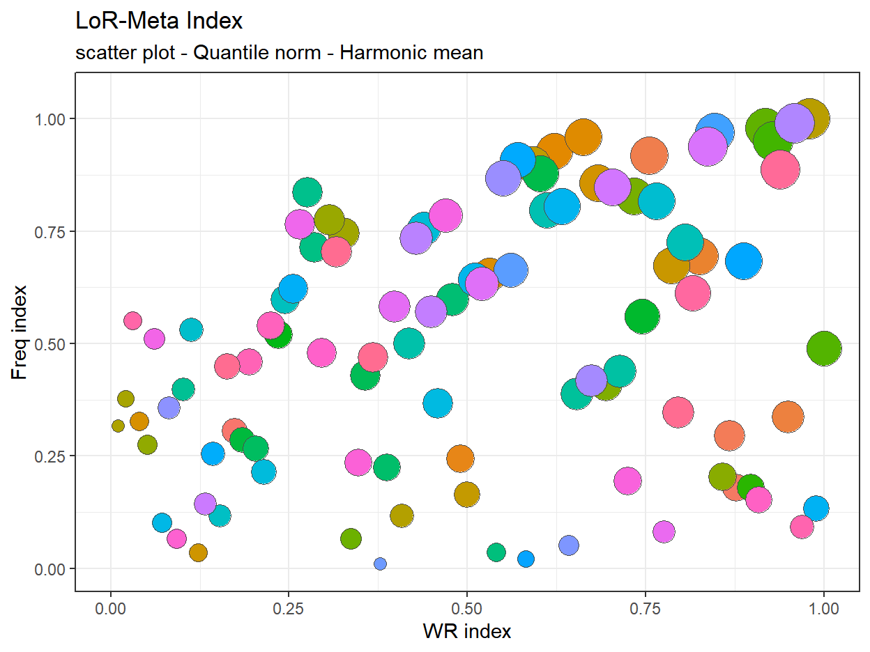
Figure 11: LMI / filter at 200 / Quantile normalization / Harmonic mean
Ranking methods
The remaining steps are related to the validation of an Index, the visualization process and other quality checks, the aggregation was the last steps of the “computation phase”. This “quality checks” are a vast topic but it’s not really necessary for such simple CI. So, now, as mentioned right before the aggregation step, I’ want to I’ll try to use a different approach to Normalization and Aggregation: working with ranks. It means that the variable are reduced to their ranking order. Of course this is only possibles with variables that can be ordered, so for example not with most categorical data. The order of course doesn’t have to be from the max to the min, it depends of the correlation between the variables and the objective of the Index. For example if we won’t an “Environmental Index”, CO2 levels can be ranked from the min to the max. Transforming the direction of a variable can be used also in the previous context but here it’s as, if not more important. I’ll only introduce one ranking method: Borda ranking method.
Aggregating Ranks: Borda
The method is quite simple: first of all, for each item in a variable we assign a value corresponding at how high the item is ranked.
Example If we have 5 values for the variable X: (0.6,0.4,1,0,0.2) their ranking is -> (2,3,1,5,4) -> if we give 0 point to the min value, 1 to the second to last and so on until N-1 (with N the number of values of X) we have the result points -> (3,2,4,0,1). In order to improve a little the results and readability I’ll change a little the rules by giving from 1 to N points.
We repeat this for each variable and then we sums the point by rows.
It’s also possible to aggregate ranks simply by computing their mean / median. There are also more complex method like Copeland, CKYL but they are “wasted” with only two variables. In case this Index is expanded in the future I may try to use them.
As usual the results can be consulted in the Appendix ??
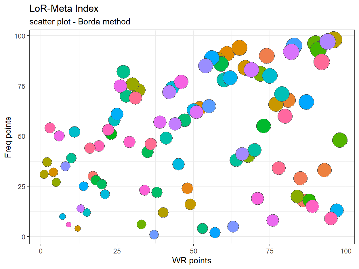
Figure 12: LMI / filter at 200 / Borda method
Fig.12 is the only case it this case study where we can’t maintain the same axis range as we are dealing with the ranks. Also, here it’s possible to understand why I decided to assign N and not N-1 point to the first ranked, so that the theoretical best deck would be at coordinate (N,N) instead of (N-1,N-1) which would have been a bit less intuitive. it also mean that the worst theoretical deck instead of being at (0,0) now it would be at (1,1).
If the plot seems similar to the Quantile one (11) it’s because it is, the quantile normalization is pretty much a conversion to the ranks. Does it means that they are equal? No. There are advantage and disadvantage for each choice. Personally I would give an edge to the Quantile and the other (not-ranbking methods) as there are more options when using a linear scale.
LMI (final)
As explained in the previous steps, to compute the LMI I currently decide to use the following methodology:
- Filtering data with less than 200 games
- Using the variables: Win Rates / Play Rate
- Quantile normalization
- Harmonic Mean as aggregation
The result is the following plot. In this case it’s possible to hover on each point to see their values. I also modified the range of the points’ radius to accentuate the differences.
And of course the data in a tabular format, ordered by decreasing LMI.
To conclude, I hope this work can be a foundation for more elaborate discussions and think how the index can be improved / expanded. The Riot API may not provide a lot of data, but there is still already so much can be done.
Appendix
Table 1: Data no Filter games
Table 2: Data filtered of decks without at least 200 games
Table 2: Data no Normalization
Table 3: Minmax table
Table 4: Quantile table
Table 5: Aggregation table
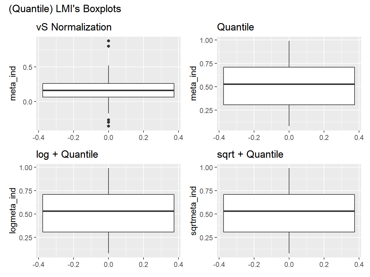
Figure 13: Boxplot of LMI when applying: vS / quantile / minmax+log trasnformation to playrate / minmax+sqrt transformation to playrate
The following is the table of the data I used for this analysis. I already filtered the cases with less than 100 games.